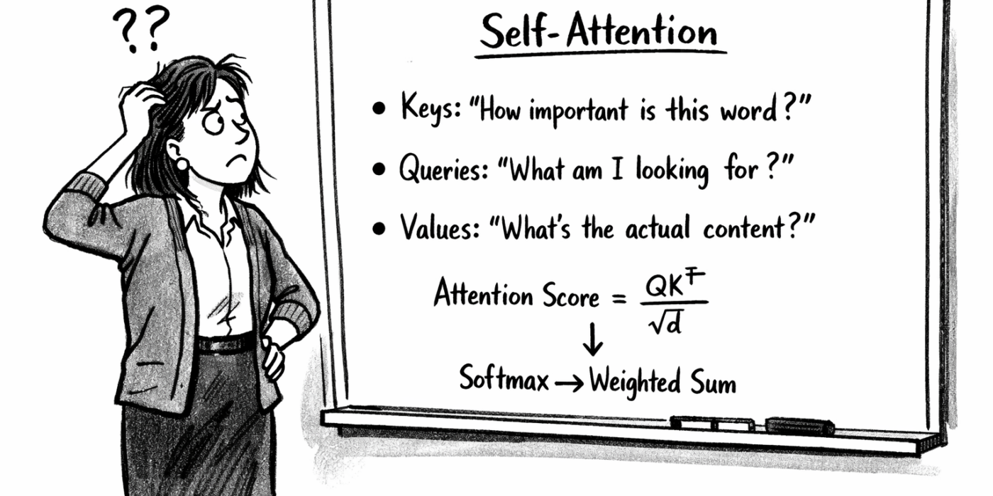
Sick of keys, queries and other cliched metaphors?
The most difficult part of the Transformer architecture to get an intuitive understanding of is self-attention. If I have to read another article on self-attention that explains about keys, queries and values – I will projectile vomit. Sorry, but it’s true.
So here’s my attempt to explains things a little more clearly. I’m assuming most people reading this have an intuitive understanding of the old RNNs, embeddings and positional encodings. If you don’t understand these somewhat, have a browse of articles about them. There are loads that explain them well.
Thanks for reading Alexis’s Substack! Subscribe for free to receive new posts and support my work.
Token embeddings – fake, for illustration
In real models, embeddings are 768 or 4096 dimensions. Here I’m using 2D so you can see actual numbers. These values are made up – the point is just to have concrete vectors to work with.
The / the: [0.30, 0.80]
cat: [1.00, 0.50]
sat: [0.70, 0.90]
on: [0.20, 0.30]
Brian: [0.60, 0.40]
typed: [0.50, 0.70]
into: [0.30, 0.40]
Is: [0.40, 0.60]
your: [0.30, 0.50]
warm: [0.80, 0.30]
black: [0.20, 0.70]
What embeddings do
Before any of this, the network learns a vector for each word in its vocabulary. Words that function similarly end up with vectors pointing in similar directions.
“”cat,” “dog,” “hamster” → nearby vectors (all pets, all nouns, all can sit/run/eat)
“typed,” “wrote,” “entered” → nearby vectors (all input actions, all past tense)
“warm,” “cold,” “hot” → nearby vectors (all temperature descriptors)
“cat” and “typed” end up far apart – they share almost no grammatical or semantic role.
This happens automatically through training. Words that can substitute for each other in many contexts get gradients that push their embeddings together.
Measuring similarity with dot product
The dot product of two vectors is highest when they point in the same direction, zero when perpendicular, negative when opposing.
Geometrically: it measures “how much does vector A go in the same direction as vector B?”
[1, 0] · [1, 0] = 1 (identical directions, maximum similarity)
[1, 0] · [0, 1] = 0 (perpendicular, no similarity)
[1, 0] · [-1, 0] = -1 (opposite directions, maximum dissimilarity)
So if we want to measure “how similar are these two vectors,” dot product is a cheap, differentiable way to do it.
Why positional encodings exist
In an RNN, order is implicit: position 3’s hidden state was computed from position 2’s, which came from position 1’s. The architecture enforces sequence.
Self-attention has no such structure. Every position is processed in parallel, and nothing in the dot product machinery distinguishes “cat sat” from “sat cat” – the same embeddings, the same arithmetic.
So the model needs order information injected explicitly. We add a different vector to each position, nudging identical words at different positions into different regions of the space.
Positional encodings – fake, for illustration
pos_0: [0.10, 0.00]
pos_1: [0.00, 0.10]
pos_2: [0.10, 0.10]
pos_3: [0.00, 0.20]
pos_4: [0.20, 0.00]
The addition step
Every token gets its embedding added element-wise to its position’s encoding:
“The” at position 0: [0.30, 0.80] + [0.10, 0.00] = [0.40, 0.80]
“cat” at position 1: [1.00, 0.50] + [0.00, 0.10] = [1.00, 0.60]
These combined vectors are what enter the rest of the network. The word’s meaning and its position get fused into one vector from this point forward.
Three phrases, fully positioned
Phrase 1: “The cat sat on the” → predict “mat”
Position 0: “The” → [0.40, 0.80]
Position 1: “cat” → [1.00, 0.60]
Position 2: “sat” → [0.80, 1.00]
Position 3: “on” → [0.20, 0.50]
Position 4: “the” → [0.50, 0.80]
Phrase 2: “Brian typed cat into the” → predict “terminal”
Position 0: “Brian” → [0.70, 0.40]
Position 1: “typed” → [0.50, 0.80]
Position 2: “cat” → [1.10, 0.60]
Position 3: “into” → [0.30, 0.60]
Position 4: “the” → [0.50, 0.80]
Phrase 3: “Is your warm black cat” → predict “happy”
Position 0: “Is” → [0.50, 0.60]
Position 1: “your” → [0.30, 0.60]
Position 2: “warm” → [0.90, 0.40]
Position 3: “black” → [0.20, 0.90]
Position 4: “cat” → [1.20, 0.50]
“cat” is now three different vectors
Phrase 1, position 1: [1.00, 0.60]
Phrase 2, position 2: [1.10, 0.60]
Phrase 3, position 4: [1.20, 0.50]
Same word. Different inputs to the network.
The network should learn which other words are relevant
Transformers gain great power from learning which words are relevant to which.
For predicting “mat”: the network benefits when “cat” aligns strongly with “sat”. The rhyme and physical setup (”cat sat on…mat”) matters.
If instead “cat” aligned with “on” or “the”, the model loses the rhyming cue and the specific action. “on the” could precede almost anything – ”table,” “floor,” “roof.” The prediction becomes generic. Worse: if “cat” aligned only with itself (ignoring context entirely), it might predict “food” or “nap” – things cats are associated with, but wrong for this phrase.
For predicting “terminal”: the network benefits when “cat” aligns strongly with “typed” and “Brian”. This is command-line context – someone typing a command.
If instead “cat” aligned with “into” and “the”, the model sees only generic function words. “cat into the” could end with “room,” “box,” “carrier” – a physical cat going somewhere. The technical context vanishes. The human name “Brian” and the action “typed” are what signal this is about computers, not animals.
For predicting “happy”: the network benefits when “cat” aligns strongly with “Is,” “warm,” and “black”. It’s a question about the state of a cat with certain attributes.
If instead “cat” aligned only with “your”, the model knows there’s possession but misses that it’s a question (from “Is”) and misses the descriptive context (from “warm,” “black”). It might predict “outside” or “here” – reasonable continuations for “your cat” but wrong for a question about emotional state. The word “Is” at position 0 is critical: it transforms “your warm black cat” from a noun phrase into an inquiry requiring an adjective response.
Relevance is learned, not predefined
Nothing in the raw embeddings or positional encodings encodes “sat is relevant to cat in this context.” The network doesn’t start knowing what relevance means.
Instead, relevance gets baked into two learned matrices during training. Call them W_search and W_offer. These matrices transform positioned embeddings into a new space where dot product corresponds to relevance.
Before training: random matrices, dot products are meaningless
After training: matrices have been adjusted so that dot products between transformed vectors produce useful relevance patterns.
The “knowledge” of what should align with what lives entirely in the learned weights of these two matrices.
What the relevance matrices must achieve – the heart of self-attention
The two matrices are designed to work together like this: if word A is relevant to word B in some context, then A transformed by W_search should be similar to B transformed by W_offer. Similar transformations → high dot product → strong alignment.
So the problem becomes: learn W_search and W_offer such that, for every useful relevance relationship across all training data, the transformed vectors end up pointing in similar directions.
Concretely:
When “cat” is at position 1 in “The cat sat on the”:
“cat” transformed by W_search must be similar to “sat” transformed by W_offer
Because alignment with “sat” helps predict “mat”
When “cat” is at position 2 in “Brian typed cat into the”:
“cat” transformed by W_search must be similar to “typed” transformed by W_offer
Because alignment with “typed” helps predict “terminal”
When “cat” is at position 4 in “Is your warm black cat”:
“cat” transformed by W_search must be similar to “Is” transformed by W_offer
Because alignment with “Is” helps predict “happy”
The small positional differences ([1.00, 0.60] vs [1.10, 0.60] vs [1.20, 0.50]) must result in W_search transformations that are similar to completely different W_offer transformations.
How the network computes alignment
Every positioned embedding gets multiplied by both relevance matrices, producing two vectors per position:
(positioned embedding) × W_search → one vector
(positioned embedding) × W_offer → another vector
To compute how strongly position j aligns with position i:
1. Take position i’s W_search transformation
2. Take position j’s W_offer transformation
3. Dot product gives a score
4. After softmax across all j, this score becomes a weight
5. Position i’s new representation is the weighted sum of all positions’ embeddings, weighted by these alignment scores
No word “decides” anything. The matrices are fixed (after training), the dot product is just arithmetic, and the alignments are determined entirely by which transformations happen to be similar.
Training adjusts W_search and W_offer until the similarities produce alignment patterns that reduce prediction error.
Why this seems impossible but works
In 2D, there’s almost no room to manoeuvre. The positional nudges are tiny compared to what’s being asked.
In real models (768D, 4096D), there’s vastly more geometric room. The positional encoding can push the W_search transformation into a subspace where “sat”-like W_offer transformations are similar, or a different subspace where “typed”-like W_offer transformations are similar. The curse of dimensionality becomes a blessing – there are enough nearly-orthogonal directions to encode many different alignment patterns without interference.
[And yes – W_offer and W_search do correspond to those Query and Key matrices in traditional explanations of self-attention – Alexis]
Another way to think of W_offer and W_search
Self-attention is a weighted average over the past
That sentence hides the important bit, so let’s unpack it.
For a given token at position t:
- Compute a weight for every previous position
- Take the weighted sum of their representations
- That sum becomes the new representation at position t
Mathematically: output(t) = Σᵢ weight(t, i) × representation(i)
That’s it. A weighted average.
A naive average treats all previous positions equally. Self-attention doesn’t:
- The weights are content-dependent. Different tokens produce different weights. “cat” in one context might weight “sat” heavily; in another context it might weight “typed” heavily.
- The weights are sharply non-uniform. Softmax concentrates mass on a few positions. Most tokens contribute almost nothing.
So while the mechanism is averaging, the effect is selective combination.
From bigrams to self-attention
Bigram: position t looks only at position t-1. Fixed window (N=2), no learned relevance.
N-gram: position t looks at positions t-1, t-2, … t-N. Larger fixed window, but still no content-dependent weighting.
Self-attention: position t looks at all previous positions, with weights computed from content. Variable window, learned relevance.
Self-attention is what you get when you ask: “What if we let each position decide how much to weight every previous position, based on what’s actually there?”